v24.03, tested for GrADS v2.2.1 on Linux.
| Script |
Usage (<>: required arguments; [<>]: optional arguments) |
Gallery |
|
deseason.gs
|
Calculate climatological mean or anomalies.

USAGE 1: deseason -v <var1> [<var2>...] [-a <anom1> [<anom2>...]] [-l <limit_start> <limit_end>] [-n <num_Fourier>] [-u <undef>] [-o <file>] [-p <path>]
USAGE 2: deseason -v <var1> [<var2>...] -c <clim1> [<clim2>...] [-l <limit_start> <limit_end>] [-n <num_Fourier>] [-u <undef>] [-o <file>] [-p <path>]
  <var>: input field. Can be any GrADS expression.
  <anom>: anomaly. Default=<var>.
  <clim>: climatology.
  <limit_start> <limit_end>: climatology is calculated using data over the period of <limit_start> to <limit_end> only. Specified in world coordinate, such as MMMYYYY.
  <num_Fourier>: if unset, climatology is defined as long-term mean seasonal cycle; if set, climatology is further smoothed using first <num_Fourier> Fourier harmonics
                 (i.e., annual, biannual, triannual, etc.) plus mean. (Smoothing is recommended if the number of years is not sufficiently large.)
  <undef>: undef value for .dat and .ctl. Default=-9.99e8.
  <file>: common name for output .dat and .ctl files. If set, no variable is defined, only file output.
  <path>: path to output files. Do NOT include trailing "/". Current path is used if unset.

NOTE: regular and 365-day calendars are supported and automatically handled. For regular calendar, a climatological year is assumed to be 365.2425 days.

EXAMPLE 1: calculate SST climatology and save to variable "sstclim" (no file output).
  deseason -v sst -c sstclim

EXAMPLE 2: as example 1 except save to files "sstclim.ctl" and "sstclim.dat" (no variable is defined).
  deseason -v sst -c sstclim -o sstclim

EXAMPLE 3: as example 1 except climatology is further smoothed using first 4 Fourier harmonics (i.e., annual, biannual, triannual, and quarterly) plus mean.
  deseason -v sst -c sstclim -n 4

EXAMPLE 4: calculate SST anomaly and save to variable "sstanom" (no file output).
  deseason -v sst -a sstanom

DEPENDENCIES: qdims.gsf parsestr.gsf
|
|
|
drawbox.gs
|
Draw an unfilled "box" under any map projection.

Usage: drawbox <lon1> <lon2> <lat1> <lat2>
  <lon1>: Beginning longitude.
  <lon2>: Ending longitude. Must be >= <lon1>.
  <lat1>: Beginning latitude.
  <lat2>: Ending latitude. Must be >= <lat1>.
|
 Guan et al. (2014), Fig. 2 left
|
|
drawline.gs
|
Draw lines at specified locations.

USAGE: drawline Lon|Lat|Lev|Val|Time <coordinate1> [<coordinate2>...] [Lon|Lat|Lev|Val|Time <coordinate1> [<coordinate2>...]]...
  <coordinate>: world coordinate.

EXAMPLE 1: drawline Lon 180 Lat 0
  Draw international date line and equator on a map.

EXAMPLE 2: drawline Val -1 0 1
  Draw lines with constant value -1, 0 and 1 in a line graph.

EXAMPLE 3: drawline Time 1Jan2005
  Draw a straight line marking 1 January 2005.

NOTE: proper capitalization MUST be used for key words Lon, Lat, Lev, Val and Time.
|
 Guan and Nigam (2009), Fig. 1
|
|
drawmark.gs
|
Draw marks at data points of a 2-D field.

USAGE: drawmark <var> <mark> <color1>[&<color2>] <size> [<magnitude> [<append> [<text>]]]]
  <var>: variable name. Can be any GrADS expression.
  <mark>: mark type.
  <color>: mark color. <color1>=negative, and <color2>=positive if two colors are given.
  <size>: reference mark size (diameter).
  <magnitude>: mark sizes (diameters) are set proportional to square root of variable magnitude if <magnitude> is nonzero, or <size> if zero. Default=0.
  <append>: 0 (default) or 1. Set to 1 if appending to an existing plot. (Run "legend.gs" after all data are plotted.)
  <text>: Text to be shown in legend. Text beginning with a minus sign or containing spaces must be double quoted.

NOTE: <var> must be on a grid consistent with default file. If not, use "set dfile" to change default file.

EXAMPLE 1:
  drawmark swe 3 3 0.1 0.5
  legend

EXAMPLE 2:
  drawmark sat-273.15 3 4&2 0.1 5
  legend

DEPENDENCIES: qdims.gsf

SEE ALSO: legend.gs
|
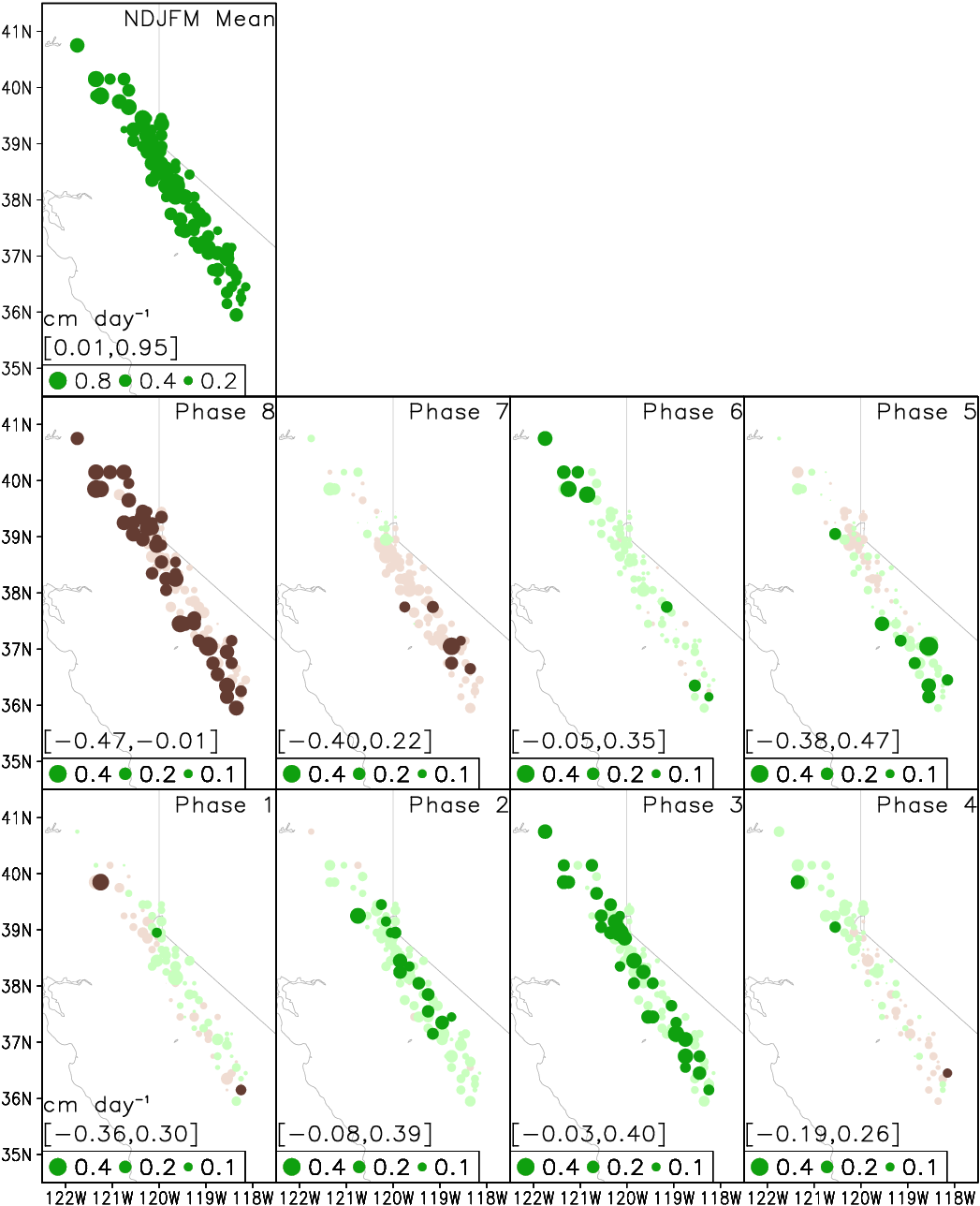 Guan et al. (2012), Fig. 7
|
|
drawstr.gs
|
Annotate current plot.

USAGE 1: drawstr -t <text1> [<text2>...] [-p <position1> [<position2>...]] [-c <color1> [<color2>...]] [-z <size1> [<size2>...]]
         [-k <thickness1> [<thickness2>...]] [-b <background1> [<background2>...]] [-xo <xoffset1> [<xoffset2>...]] [-yo <yoffset1> [<yoffset2>...]]
USAGE 2: drawstr -T <TEXT1> [<TEXT2>...] [-p <position1> [<position2>...]] [-c <color1> [<color2>...]] [-z <size1> [<size2>...]]
         [-k <thickness1> [<thickness2>...]] [-xo <xoffset1> [<xoffset2>...]] [-yo <yoffset1> [<yoffset2>...]]
  <text>: label for an individual panel. Text beginning with a minus sign or containing spaces must be double quoted.
  <TEXT>: label for a multi-panel plot (e.g., main title, column title, etc.). Text beginning with a minus sign or containing spaces must be double quoted.
  <position>: position of <text> or <TEXT>.
              For <text>, refer to schematic below. For <TEXT>, use <idx>t|b|l|r, where <idx> is from subplot.gs and t|b|l|r refers to top|bottom|left|right.
              Default="1 2 3..." for <text>, and "1t 2t 3t..." for <TEXT>.
  <color>: text color. Default=1.
  <size>: text size. Current setting is used for <text> if unset. Default=0.18 for <TEXT>.
  <thickness>: text thickness.
  <background>: background color of text. Applicable to text inside plotting area only.
  <xoffset>: horizontal offset to default position. Default=0.
  <yoffset>: vertical offset to default position. Default=0.

               <TEXT>

  1               2               3
  +-------------------------------+
  |11                           12|
  |                               |
  |                               |
 9|           Plot Area           |10
  |                               |
  |                               |
  |4                             5|
  +-------------------------------+
          7       6       8

NOTE: "-T" and "-t" options cannot be used together.

EXAMPLE 1: add axis labels.
  drawstr -p 6 9 -t Longitude Latitude

EXAMPLE 2: add column titles for a 3 rows by 2 columns plot.
  subplot 6 1
  ...
  subplot 6 6
  ...
  drawstr -p 1t 4t -T "Column A" "Column B"

DEPENDENCIES: parsestr.gsf
|
 Guan et al. (2012), Fig. 2
|
|
hist.gs
|
Calculate histogram.

USAGE: hist t|xy <input> <output> <left_edge> <right_edge> <bin_size>
  t|xy: statistics are calculated over selected dimension(s).
  <input>: input field (can have horizontal dimensions; NO vertical dimension).
  <output>: histogram.
  <left_edge>: left edge.
  <right_edge>: right edge.
  <bin_size>: bin size.

EXAMPLE 1: histogram over time.
  set time Jan1901 Dec2000
  hist t precip preciphist -2 2 0.25
  set time Jan1901
  set lev -2 2
  set xyrev on
  display preciphist

EXAMPLE 2: histogram over space.
  set lon 0 360
  set lat -90 90
  hist xy precip preciphist -2 2 0.25
  set lon 0
  set lat 0
  set lev -2 2
  set xyrev on
  display preciphist

DEPENDENCIES: qdims.gsf
|
|
|
import.gs
|
Import time series from text file.

USAGE: import -v <var1> [<var2>...] -i <file> [-rows <row_start>] [-rowe <row_end>] [-col <column1> [<column2>...]] [-u <undef>] [-t0 <time_start>] [-dt <step>]
  <var>: variable to be imported.
  <file>: input file containing time series (one variable per column). Non-numeric values are treated as missing value flags.
  <row_start>: row number of first row to read. Default=1 (beginning of file).
  <row_end>: row number of last row to read. Read to end of file if unset.
  <column>: column number for each variable. Default="1 2 3...".
  <undef>: missing value flag in <file>.
  <time_start>: time corresponding to <row_start>. Specified in world coordinate, such as MMMYYYY. Ignored and matched to current time dimension if the latter is already set.
  <step>: time step between each row, e.g., 6hr, 5dy, 3mo, 1yr, etc. Ignored and matched to current time dimension if the latter is already set.

EXAMPLE 1: import daily PNA index from "PNA_Daily.txt" where the first row corresponds to 1JAN1950, and missing values are flagged -9999.
  import -v pna -i PNA_Daily.txt -u -9999 -t0 1JAN1950 -dt 1dy

EXAMPLE 2: as above, but with another daily file already open.
  set time 1JAN1950
  import -v pna -i PNA_Daily.txt -u -9999

DEPENDENCIES: parsestr.gsf qdims.gsf
|
|
|
lanczos.gs
|
Apply Lanczos filter in time dimension.

USAGE: lanczos -v <var1> [<var2>...] [-n <name1> [<name2>...]] [-c <period1> [<period2>]] [-w <num_weight>] [-u <undef>] [-o <file>] [-p <path>]
   <var>: input variable. Can be any GrADS expression with NO missing values.
   <name>: name for output variable. Same as <var> if unset.
   <period>: cutoff period(s) specified in # of time steps; one argument for lowpass filtering, two arguments for bandpass filtering (order of arguments does not matter).
   <num_weight>: # of weights on each side (a total of 2*<num_weight>+1 weights will be used). Default=<period>.
   <undef>: undef value for .dat and .ctl. Default=-9.99e8.
   <file>: common name for output .dat and .ctl files. If set, no variable is defined, only file output.
   <path>: path to output files. Do NOT include trailing "/". Current path is used if unset.

DEPENDENCIES: parsestr.gsf qdims.gsf
|
|
|
legend.gs
|
Draw legend for current plot.

USAGE 1: legend colorbar [-orient v|h] [-xo <xoffset>] [-yo <yoffset>] [-scale <scalefactor>] [-u <unit>]
USAGE 2: legend [-orient v|h] [-xo <xoffset>] [-yo <yoffset>] [-scale <scalefactor>] [-u <unit>]
  colorbar: for shading plot.
  v|h: v=vertically oriented (default), h=horizontally oriented.
  <xoffset>: horizontal offset to default position. Default=0.
  <yoffset>: vertical offset to default position. Default=0.
  <scalefactor>: scale factor for line length and space. Default=1.
  <unit>: unit label placed near legend for shading or mark plot.

DEPENDENCIES: parsestr.gsf

SEE ALSO: shadcon.gs drawmark.gs plot.gs taylor.gs vector.gs
|
|
|
ltrend.gs
|
Calculate linear trend over time (based on least-squares fitting).

USAGE: ltrend <input> [<output> [<slope> [<rmse>]]]
  <input>: input field. Can be any GrADS expression.
  <output>: output field, i.e., fitted trend line. Default=<input>.
  <slope>: slope of fitted trend line, i.e., change of <input> per time step.
  <rmse>: root mean square error.

DEPENDENCIES: qdims.gsf
|
|
|
monmask.gs
|
Create mask for specified calendar months.

USAGE: monmask <start> <end> <mask> [<month>]
  <start> <end>: range of calendar month(s) NOT to mask out.
  <mask>: mask. Ones over <start> to <end> inclusive, missing values elsewhere.
  <month>: calendar month where <mask> = 1, missing value elsewhere.

NOTE: any time grid or calendar is supported.

EXAMPLE 1: define a variable "winmask" with ones over December, January, and February, and missing values over other months.
  monmask 12 2 winmask

EXAMPLE 2: define a variable "summask" with ones over June, July, and August, and missing values over other months.
  monmask 6 8 summask

EXAMPLE 3: define a variable "julmask" with ones over July and missing values over other months.
  monmask 7 7 julmask

DEPENDENCIES: qdims.gsf
|
|
|
norm.gs
|
Normalize in time dimension.

USAGE: norm <input> [<output> [<mean> [<std> [<base_period_start> [<base_period_end>]]]]]
  <input>: input time series.
  <output>: output time series. Defalt=<input>.
  <mean>: sample mean.
  <std>: sample standard deviation.
  <base_period_start> <base_period_end>: period for calculating <mean> and <std>. Specified in world coordinate, e.g., Jan1960.

DEPENDENCIES: qdims.gsf
|
|
|
one2one.gs
|
Apply one-two-one smoothing in time dimension.

USAGE: one2one <input> [<output> [<iterations> [<option>]]]
  <input>: input field.
  <output>: output field. Default=<input>.
  <iterations>: number of iterations. Default=1. No smoothing will be performed if <= 0.
  <option>: set to "interannual" to smooth over same calendar months/seasons."
|
 Guan and Nigam (2008), Fig. 2
|
|
parsestr.gsf
|
Ancillary script.
|
|
|
plot.gs
|
Plot 1-D graph.
USAGE: plot -v <var1> [<var2>...] [-r <range_from> <range_to>] [-m <mark1> [<mark2>...]] [-z <size1> [<size2>...]] [-s <style1> [<style2>...]]
[-c <color1> [<color2>...]] [-k <thick1> [<thick2>...]] [-t <text1> [<text2>...]] [-append 1]
<var>: variable to be plotted.
<range_from> <range_to>: axis limit. Minimum and maximum values are used if unset.
<mark>: mark type. Default="2 3 4...", i.e., open circle, closed circle, open square, closed square, etc.
<size>: mark size. Default=0.11,
<style>: line style. Current setting is used if unset.
<color>: mark/line color. Default="1 2 3...", i.e., foreground color, red, green, dark blue, etc.
<thick>: mark/line thickness. Integers between 1 and 12. Current setting is used if unset.
<text>: text to be shown in legend. Text beginning with a minus sign or containing spaces must be double quoted.
-append 1: use if appending to an existing plot. (Run "legend.gs" only once after all data are plotted.)
EXAMPLE 1: plot three variables with lines.
plot -v ao pna nino34 -t AO PNA Nino3.4"
legend
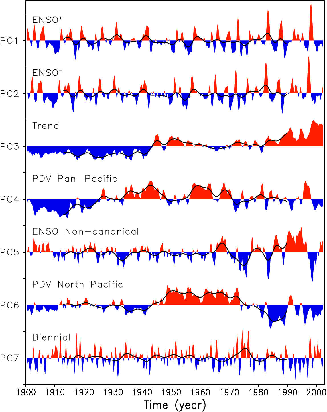
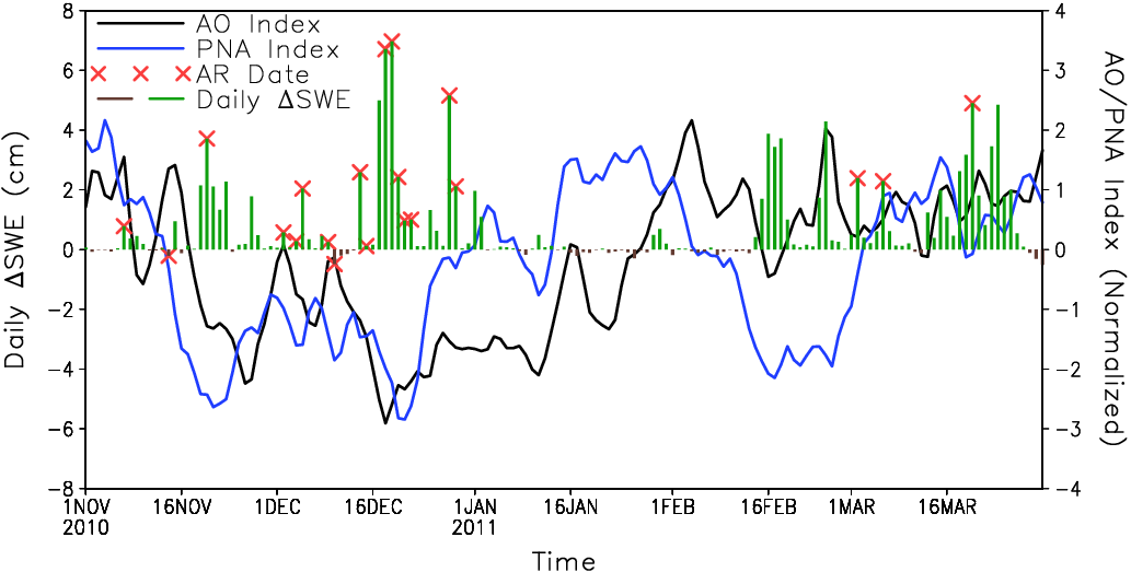
EXAMPLE 2: plot one variable with 2-colored bars based on signs and another variable with line.
zeros=0
plot -v ao;zeros pna -t AO PNA -s bar 1 -k 10 5 -c 2;4 1
legend
DEPENDENCIES: parsestr.gsf
SEE ALSO: legend.gs
|
 Guan et al. (2013), Fig. 5
|
|
ppp.gs
|
Produce properly-cropped, publication-ready graphic files.

USAGE: ppp <outfile> [<format1>] [<format2>]...
  <outfile>: full path of output file. Do NOT include the filename extension (e.g., use "mypath/myfile", instead of "mypath/myfile.eps").
  <format>: eps (default), pdf, or png.

EXAMPLE 1: print to "myfile.eps".
  ppp myfile

EXAMPLE 2: print to "myfile.png".
  ppp myfile png
|
|
|
qdims.gsf
|
Ancillary script.
|
|
|
rebin.gs
|
Compress/expand data temporally and/or horizontally (e.g., convert data at daily intervals to monthly or vice versa).

USAGE: rebin -v <var1> [<var2>...] [-n <name1> [<name2>...]] [-d <description1> [<description2>]]
       [-t <step>] [-xy <nx> <lon_start> <dlon> <ny> <lat_start> <dlat>] [-m <method>] [-u <undef>] [-o <file>] [-p <path>]
  <var>: input variable. Can be any GrADS expression.
  <name>: name for output variable. Same as <var> if unset.
  <description>: description (long name) for a variable. <var> is used if unset.
  <step>: time interval of rebinned data. MUST be specified in world coordinate, e.g., 6hr, 5dy, 3mo, 1yr, etc. No temporal rebinning if unset.
  <nx>...<dlat>: arguments for horizontal rebinning. Box averaging (bilinear interpolation) is used when converting to coarser (finer) grid. No horizontal rebinning if unset.
  <method>: method for temporal compression (ave, sum, min, max, or skip). Default=ave. (Repeating is used in case of temporal expansion and is the only method supported.)
  <undef>: undef value for .dat and .ctl. Default=-9.99e8.
  <file>: common name for output .dat and .ctl files. If set, no variable is defined, only file output.
  <path>: path to output files. Do NOT include trailing "/". Current path is used if unset.

NOTE: rebinning starts exactly at the first time step of the current dimension, and ends at or before the last time step of the current dimension.
      E.g., if input is 6-hourly, time is set to 06Z01JAN2000-18Z31JAN2000, and <step>=1dy, then rebinning starts at 06Z01JAN2000, and ends at 00Z31JAN2000.

EXAMPLE 1: create weekly mean and save to variable "sstweek".
  set time 01JAN2000 31DEC2010
  rebin -t 7dy -v sst -n sstweek

EXAMPLE 2: as example 1 but with horizontal rebinning as well.
  set time 01JAN2000 31DEC2010
  rebin -t 7dy -xy 144 0 2.5 73 -90 2.5 -v sst -n sstweek

EXAMPLE 3: create monthly sum and save to files "precipmon.ctl" and "precipmon.dat".
  set time 00Z01JAN2000 23Z31DEC2010
  rebin -t 1mo -v precip -m sum -o precipmon

DEPENDENCIES: parsestr.gsf qdims.gsf
|
|
|
rmean.gs
|
Apply running mean in time dimension.

USAGE 1: rmean <input> <window_size> [<output>]
USAGE 2: rmean <input> <window_start> <window_end> [<output>]

EXAMPLE 1: successively average "sst" over 4 time steps t-2, t-1, t, t+1, and save to variable "sstnew".
  rmean sst 4 sstnew

EXAMPLE 2: successively average "sst" over 3 time steps t-1, t, t+1, and save to variable "sstnew".
  rmean sst -1 1 sstnew
|
|
|
rms.gs
|
Calculate root mean squares.

USAGE: rms t|xy <input> <rms>
  t|xy: statistics are calculated over specified dimension(s).
  <input>: input field.
  <rms>: root mean squares.

DEPENDENCIES: qdims.gsf
|
|
|
save.gs
|
Save data in GrADS (.dat and .ctl) or netCDF (.nc) format.

USAGE 1: save -v <var1> [<var2>...] [-n <name1> [<name2>...]] [-d <description1> [<description2>]] [-u <undef>] -o <file> [-p <path>]
USAGE 2: save -v <var> -f netCDF [-d <description>] [-u <undef>] -o <file> [-p <path>]
  <var>: variable to be saved. Can be any GrADS expression if [-f netCDF] is not in use; must be a defined variable otherwise.
  -f netCDF: save in netCDF format. Only one DEFINED variable can be saved when this option is in use.
  <name>: name for a variable in saved .ctl file. <var> is used if unset.
  <description>: description (long name) for a variable. <var> is used if unset.
  <undef>: undef value for .dat and .ctl. Default=-9.99e8.
  <file>: output filename. Do NOT include filename extension.
  <path>: path to output files. Do NOT include trailing "/". Current path is used if unset.

EXAMPLE 1: save "nino3" and "nino4" to "myfile.dat" and "myfile.ctl".
  save -v nino3 nino4 -o myfile

EXAMPLE 2: save "sst" to "myfile.nc".
  save -v sst -o myfile -f netCDF

DEPENDENCIES: parsestr.gsf qdims.gsf
|
|
|
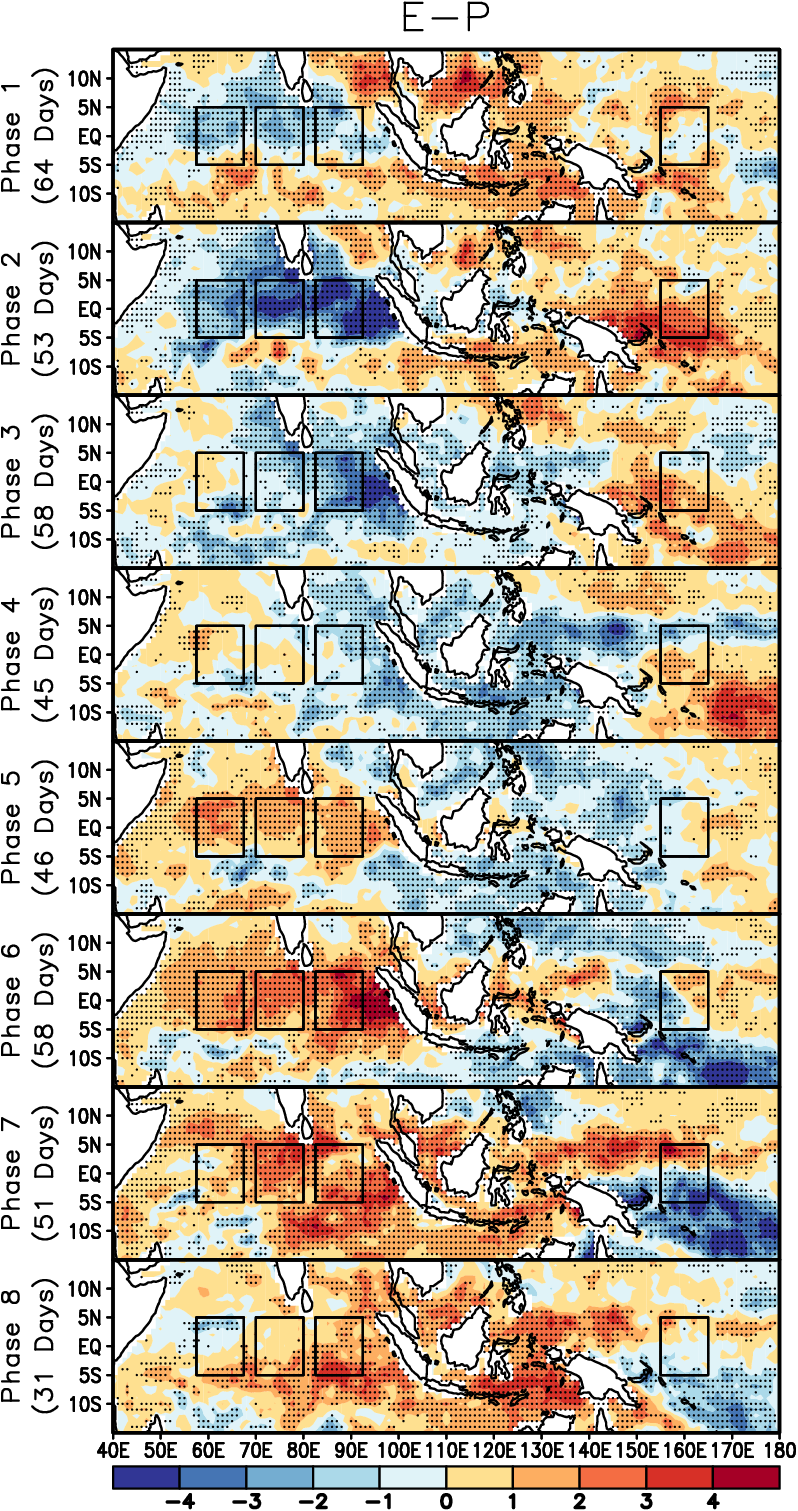
shadcon.gs
|
Plot 2-D graph using shading and/or contours with specified color and contour information.
USAGE 1: shadcon <color1>&<color2> <var> <cint> [<blackout> [grfill]]
USAGE 2: shadcon <ccolor1>[&<ccolor2>] ...
USAGE 3: shadcon <color1>&<color2>,<ccolor1>[&<ccolor2>] ...
USAGE 4: shadcon ... <offset> <var> <cint> [<blackout> [grfill]]
<color1>&<color2>: colormap for shading, e.g., blue&red. <color> can be blue, BLUE, red, or RED, and # of color levels can be specified like "blue=5". No shading if not specified.
<ccolor1>[&<ccolor2>]: color for contours below and above <offset>, e.g., 4&2. No contours if not specified.
<offset>: offset to zero for shading/contour levels. Default=0.
<var>: variable to be plotted.
<cint>: shading/contour interval.
<blackout>: values between -<blackout>*<cint> to <blackout>*<cint> will NOT be plotted.
All values will be plotted if <blackout>=0 (default).
grfill: use tiles instead of smooth contours for shading.
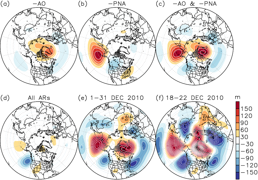
EXAMPLE 1: plot "sst" using a blue-to-red color map with a shading/contour interval of 0.1.
shadcon blue&red,1 sst 0.1
legend
EXAMPLE 2: as EXAMPLE 1, except without contours.
shadcon blue&red sst 0.1
legend
EXAMPLE 3: as EXAMPLE 2, except using grfill for shading.
shadcon blue&red sst 0.1 0 grfill
legend
EXAMPLE 4: as EXAMPLE 1, except without shading.
shadcon 1 sst 0.1
legend
|
 Guan et al. (2013), Fig. 7
|
|
subplot.gs
|
Prepare plotting area for a multi-panel plot.

USAGE: subplot <ntot> <idx> [<ncol>] [-rowmajor 0|1] [-xy <xyratio>] [-tight 0|1] [-xtight 0|1] [-ytight 0|1]
       [-xs <xspace>] [-ys <yspace>] [-xp <xpad>] [-yp <ypad>] [-x <pareawid>] [-y <pareahgt>] [-xappend 0|1] [-yappend 0|1]
  <ntot>: total number of panels to be plotted. Do NOT have to be # of rows times # of columns; will be rounded up to that value.
  <idx>: index of panel. In any column/row, panels with smaller <idx> MUST be plotted earlier.
  <ncol>: number of columns. Default=2 (even if <ntot> = 1).
  -rowmajor 1: plot 1st row first, then 2nd row, ...
  <xyratio>: aspect ratio of plotting area. Default=1. An optimal value is calculated for map projections.
  -tight 1: leave no spaces between panels.
  -xtight 1: leave no horizontal spaces between panels.
  -ytight 1: leave no vertical spaces between panels.
  <xspace>: horizontal spacing in addition to default value.
  <yspace>: vertical spacing in addition to default value.
  <xpad>: horizontal padding in addition to default value.
  <ypad>: vertical padding in addition to default value.
  <pareawid>: arbitrary parea width.
  <pareahgt>: arbitrary parea height. Ignored if <pareawid> is specified.
  -xappend 1: attach a new page right of existing plots. This is NOT intended for simple multi-column plots.
  -yappend 1: attach a new page below existing plots. This is NOT intended for simple multi-row plots.

NOTE:
  1. Spacing refers to blank space between virtual pages; can be any value.
  2. Padding refers to space between virtual page boundaries and plotting area; cannot be negative values.
  3. For best result, set desired dimensions before (instead of after) running this script.

EXAMPLE 1: 2 rows by 2 columns.
  set lon 120 300
  set lat -25 25
  set t 1
  subplot 4 1
  display sst
  ...
  set t 4
  subplot 4 4
  display sst

EXAMPLE 2: 3 rows by 1 column and no vertical spaces between panels.
  set lon 120 300
  set lat -25 25
  set t 1
  subplot 3 1 1 -ytight 1
  display sst
  ...
  set t 3
  subplot 3 3 1 -ytight 1
  display sst

DEPENDENCIES: parsestr.gsf qdims.gsf
|
 Guan et al. (2013), Fig. 9
|
|
taylor_calc.gs
|
Calculate statistics used in Taylor diagram.

USAGE: taylor_calc xyt|xy|t|xt|zt|xz <obs> <sim> <stdrat> [<corr> [<normbias>]]
  xyt|xy|t|xt|zt|xz: statistics are calculated over the selected dimension(s).
  <obs>: observation.
  <sim>: simulation.
  <stdrat>: STD ratio.
  <corr>: correlation.
  <normbias>: bias normalized by STD of <obs>.

DEPENDENCIES: qdims.gsf
|
|
|
taylor.gs
|
Plot Taylor diagram.

USAGE: taylor -s <STD1> [<STD2>...] -r <CORR1> [<CORR2>...] [-i <file>] [-rows <row_start>] [-rowe <row_end>]
       [-cols <column_STD>] [-colr <column_CORR>] [-colT <column_TEXT>] [-l <limit>] [-m <mark1> [<mark2>...]]
       [-z <size1> [<size2>...]] [-c <color1> [<color2>...]] [-t <text1> [<text2>...]] [-T <TEXT1> [<TEXT2>...]]
       [-levs <level1> [<level2>...]] [-levr <level1> [<level2>...]] [-levc <color>] [-append 1]
  <STD>: standard deviation.
  <CORR>: correlation.
  <file>: input file containing standard deviations (in one column) and correlations (in another column). Non-numeric values are treated as missing value flags.
  <row_start>: row number of first row to read. Default=1 (beginning of file).
  <row_end>: row number of last row to read. Read to end of file if unset.
  <column_STD>: column number of standard deviation column. Default=1.
  <column_CORR>: column number of correlation column. Default=2.
  <column_TEXT>: column number of legend text column.
  <limit>: limit of x/y axis. Default=2.5. A quarter circle is drawn if positive; a half circle is drawn if negative.
  <mark>: mark type. Default="2 3 4...", i.e., open circle, closed circle, open square, closed square, etc.
  <size>: mark size. Default=0.11,
  <color>: mark color. Default="1 2 3...", i.e., foreground color, red, green, dark blue, etc.
  <text>: text shown above each mark. Text beginning with a minus sign or containing spaces must be double quoted.
  <TEXT>: text shown in legend. Text beginning with a minus sign or containing spaces must be double quoted.
  <level>: contour levels drawn for <STD> and/or <CORR>. Contour level 1 is drawn by default for standard deviation.
  <color>: line color for <STD> and/or <CORR> contours. Default=1.
  -append 1: use if appending to an existing plot. (Run "legend.gs" only once after all data are plotted.)

EXAMPLE 1:
  subplot 1 1 1 -xy 1
  taylor -s 0.8 1.25 -r 0.8 0.9 -t A B -T "Model A" "Model B" -c 2 -m 2
  drawstr -p 6 9 corr -t "Standard Deviation" "Standard Deviation" Correlation
  legend

EXAMPLE 2:
  subplot 1 1 1 -xy 2
  taylor -s 0.8 1.25 -r -0.8 -0.9 -l -2.5 -t 1 2 -T "Model A" "Model B" -c 4 -m 3
  drawstr -p 6 corr -t "Standard Deviation" Correlation
  legend

EXAMPLE 3: input given by a text file "myinput.txt", where 1st column contains standard deviations, and 2nd column correlations.
  subplot 1 1 1 -xy 1
  taylor -i myinput.txt -T "Model A" "Model B" -c 2 -m 2
  drawstr -p 6 9 corr -t "Standard Deviation" "Standard Deviation" Correlation
  legend

DEPENDENCIES: parsestr.gsf qdims.gsf

SEE ALSO: legend.gs
|
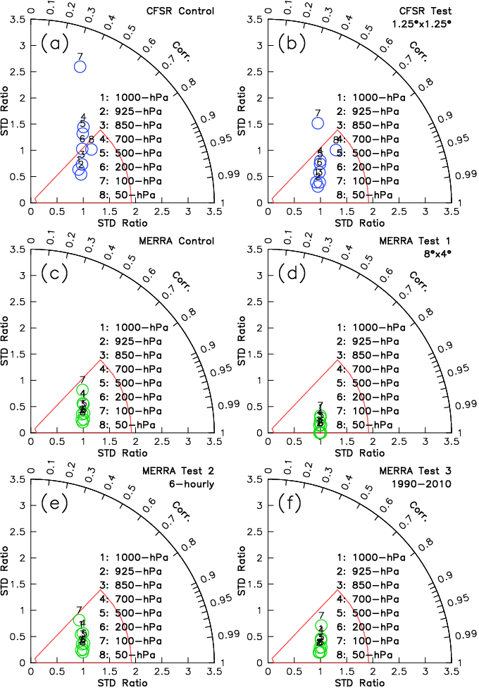 Guan et al. (2013), Fig. 9
|
|
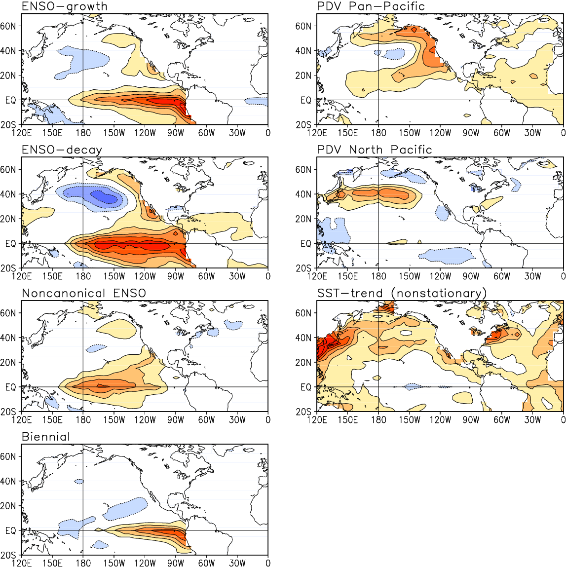
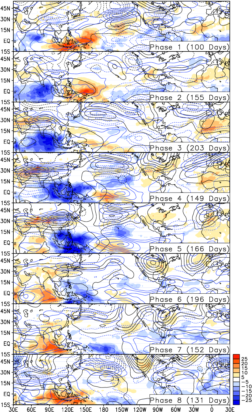
tlag.gs
|
Regress/correlate/composite with specified time lags.

USAGE: tlag regr|corr|comp <input1> <input2> <output> [<lag_start> [<lag_end>]]
  regr|corr|comp: regr for regression, corr for correlation, comp for composite.
  <input1>: independent variable, or mask for compositing (mask>=0 to include). Can be any GrADS expression. Can have a vertical dimension. Cannot have horizontal dimensions.
  <input2>: dependent variable. Can be any GrADS expression. Can have vertical and horizontal dimensions.
  <output>: output variable.
  <lag_start>: beginning lag. E.g., <lag1>=-3 for <input2> leading <input1> by 3 time steps. Default=0.
  <lag_end>: ending lag. E.g., <lag2>=3 for <input2> lagging <input2> by 3 time steps. Default=0.

NOTE 1: <input2> must be on a grid consistent with default file. If not, use "set dfile" to change default file.

NOTE 2: "set t 0" and use <output>(t+number) to get value at lag(number). E.g., <output>(t-3) gives lag regression/correlation/composite value
        when <input2> leads <input1> by 3 time steps (<input2> is shifted forward by 3 time steps for this calculation).

EXAMPLE 1: calculate and display auto-correlation function of Nino3.4 index.
  tlag corr nino34 nino34 out -24 24
  set t -24 24
  set xaxis -24 24
  display out

EXAMPLE 2: calculate and display lag regression between Nino3.4 index and global precipitation.
  tlag regr nino34 precip out -12 12
  set t 0
  subplot 8 1
  display out(t-12)
  subplot 8 2
  display out(t-8)
  subplot 8 3
  display out(t-4)
  ...
  subplot 8 7
  display out(t+12)

DEPENDENCIES: qdims.gsf
|
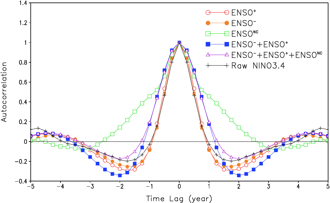 Guan and Nigam (2008), Fig. 7
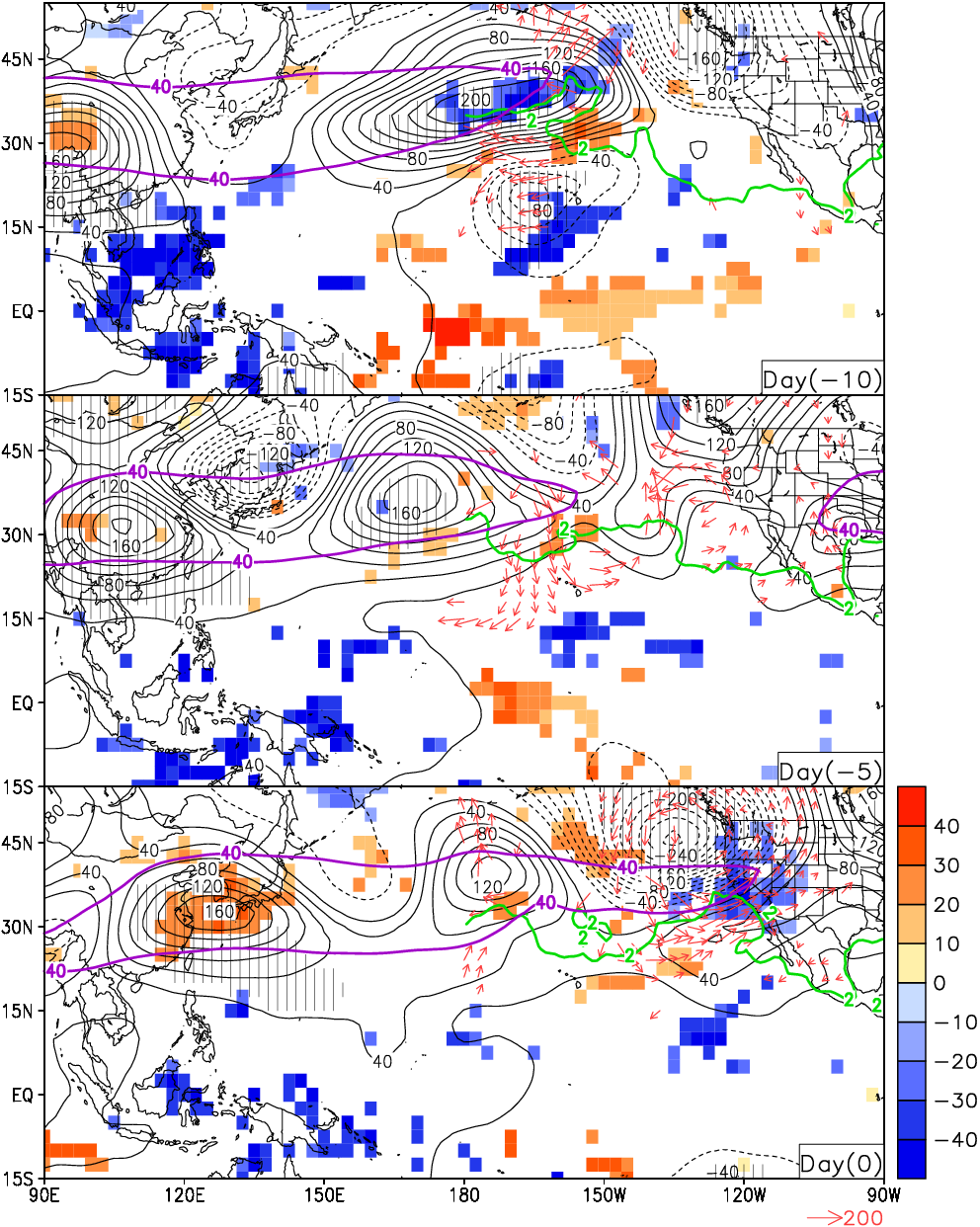 Guan et al. (2012), Fig. 5
|
|
vcr.gs
|
Create vertical cross-section.

USAGE: vcr <input> <output> [<num_point>]
  <input>: input. Can be any GrADS expression.
  <output>: vertical cross-section.
  <num_point>: set (if numeric) or return (if non-numeric) # of horizontal points sampled along cross section.

EXAMPLE:
  set lon 180 200
  set lat 15 0
  set lev 1000 100
  vcr humidity out 10
  set x 1 10
  set y 1
  set xlabs A|B
  display out

DEPENDENCIES: qdims.gsf
|
|
|
vector.gs
|
Plot vectors.
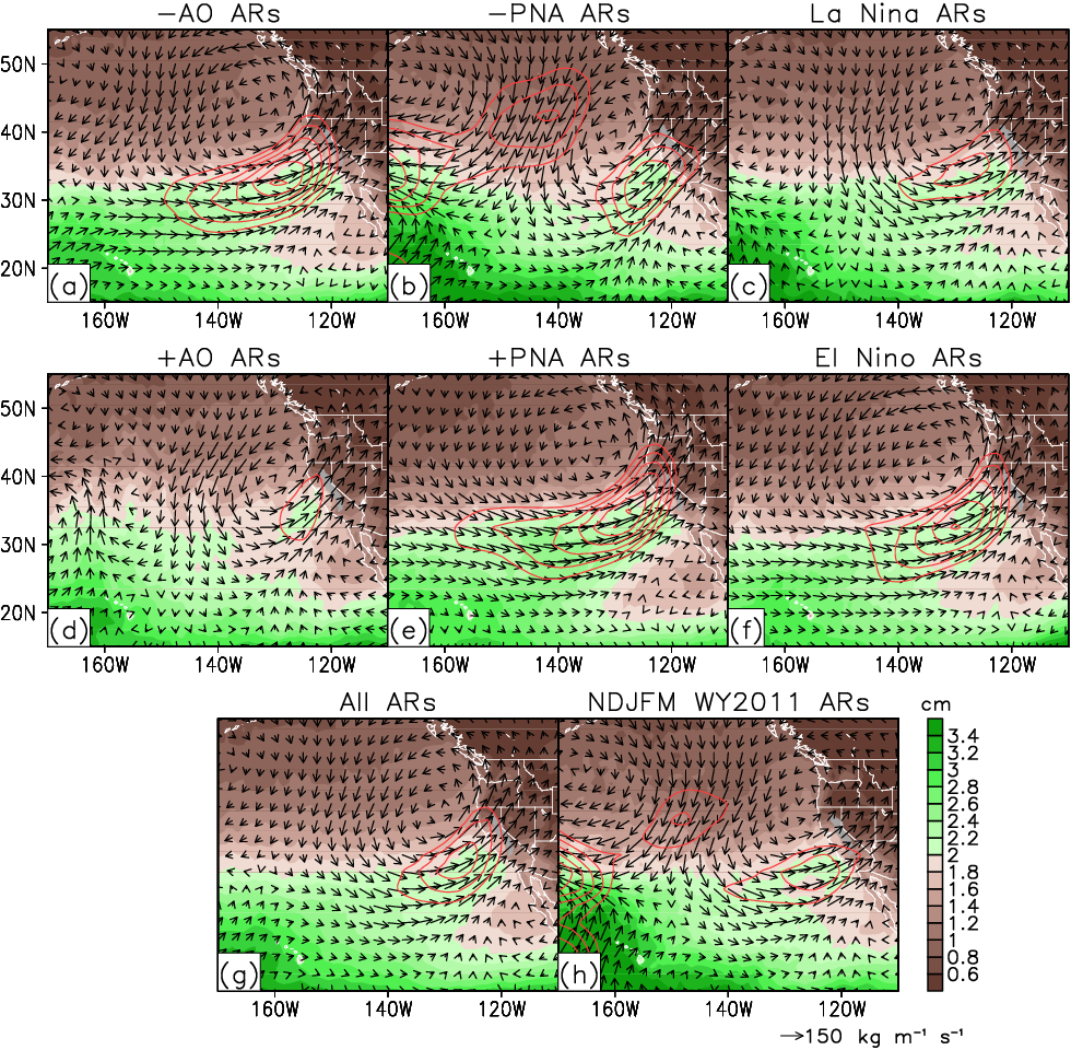
USAGE: vector <expression1>;<expression2> <length> <magnitude> [<color> [<thickness>]]
<expression1>: first component of vector.
<expression2>: second component of vector.
<length>: reference length of arrow.
<magnitude>: reference magnitude of arrow.
<color>: arrow color. Default=1.
<thickness>: arrow thickness. Default=4.
SEE ALSO: legend.gs
|
|
|
yrmask.gs
|
Create mask for specified calendar years.

USAGE: yrmask <yr1> [<yr2>...] <mask> [<year>]
  <yr>: calendar year NOT to mask out.
  <mask>: mask. Ones over unmasked years, missing values elsewhere.
  <year>: calendar year where <mask> = 1, missing value elsewhere.

NOTE: any time grid or calendar is supported.

EXAMPLE: define a variable "posIODnoENSO" with ones over 1961, 1967, and 1983, and missing values over other years.
  yrmask 1961 1967 1983 posIODnoENSO

DEPENDENCIES: qdims.gsf
|
|
|
ztest.gs
|
z-test: calculate p-value for given z.

USAGE: ztest <z> <num_tail> <p>
  <z>: z-statistic. Can be any GrADS expression.
  <num_tail>: 1 for 1-tailed test, 2 for 2-tailed test.
  <p>: p-value.
|
|